5. Analytical validation

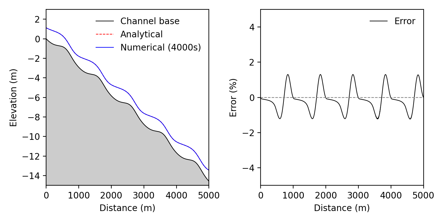
This example compares openKARST with the analytical steady-flow solution for a one-dimensional wide channel described by Delestre (2010). Further validation cases and discussion are provided in Kordilla et al. (2026).

The channel bed is constructed so that the prescribed analytical water-depth profile satisfies the steady-flow equations. The openKARST model starts from a dry channel and advances transiently toward that profile.

Complete script

The example uses 5,000 nodes and simulates 4,000 seconds, so it is substantially more computationally demanding than the preceding tutorials.

from pathlib import Path

import matplotlib.pyplot as plt
import numpy as np
import openpnm as op
from scipy.integrate import odeint
from scipy.interpolate import interp1d

from openkarst.models import FlowSimulation
from openkarst.network_generation import compute_conduit_lengths


def analytical_geometry():
    """Create the channel bed and analytical water-depth profile."""
    n_nodes = 5000
    spacing = 1.0
    x = np.linspace(0.0, 5000.0, n_nodes)

    gravity = 9.81
    discharge = 2.0
    manning = 0.03
    water_depth = 9.0 / 8.0 + 0.25 * np.sin(np.pi * x / 500.0)
    depth_interpolator = interp1d(
        x,
        water_depth,
        kind="cubic",
        fill_value="extrapolate",
    )

    def friction_slope(depth):
        return manning**2 * discharge * abs(discharge) / depth ** (10.0 / 3.0)

    def bed_slope(bed_elevation, position):
        del bed_elevation
        depth = depth_interpolator(position)
        depth_gradient = (
            np.pi / 2000.0 * np.cos(np.pi * position / 500.0)
        )
        return (
            discharge**2 / (gravity * depth**3) - 1.0
        ) * depth_gradient - friction_slope(depth)

    bed_elevation = odeint(bed_slope, [0.0], x).ravel()

    network = op.network.Cubic(
        shape=[n_nodes, 1, 1],
        connectivity=6,
        spacing=spacing,
    )
    network = compute_conduit_lengths(network)
    network["pore.coords"][:, 2] = bed_elevation

    return network, x, water_depth


def run_validation():
    network, distance, analytical_depth = analytical_geometry()

    physical_properties = {
        "water_density": 1000.0,
        "gravity": 9.81,
        "dynamic_viscosity": 0.001,
        "geometry_channel": True,
        "channel_type": "infinite",
        "channel_manning": 0.03,
    }

    solver_settings = {
        "relaxation_factor": 0.6,
        "max_iterations": 20,
        "picard_depth_tol": 1e-5,
        "ss_rel_l2tol": 1e-6,
    }

    simulation_settings = {
        "min_waterdepth": 1e-10,
        "min_flowrate": 1e-10,
        "courant": 0.8,
        "adaptive_timesteps": False,
        "dt_init": 0.1,
        "dt_max": 1.0,
        "steady_state": False,
        "t_max": 4000.0,
        "print_info_interval": 100,
    }

    output_settings = {
        "output_interval": 10.0,
        "time": True,
        "flowrates": True,
        "water_depths": True,
    }

    logging_settings = {
        "base_dir": str(Path.cwd()),
        "log_file": "analytical_validation.log",
    }

    flow = FlowSimulation(
        network,
        physical_properties=physical_properties,
        solver_settings=solver_settings,
        simulation_settings=simulation_settings,
        logging_settings=logging_settings,
    )

    flow.set_initial_conditions(
        initial_Q=np.zeros(network.Nt),
        initial_y=np.zeros(network.Np),
    )

    flow.set_inflow_BC(
        nodes=0,
        values=2.0,
        inflow_type="volumetric",
    )
    flow.set_waterdepth_BC(
        nodes=network.Np - 1,
        values=analytical_depth[-1],
    )

    results = flow.run_simulation(desired_outputs=output_settings)
    return network, distance, analytical_depth, results


def plot_comparison(network, distance, analytical_depth, results):
    bed_elevation = network["pore.coords"][:, 2]
    numerical_head = bed_elevation + results["water_depths"][-1]
    analytical_head = bed_elevation + analytical_depth

    numerical_depth = numerical_head - bed_elevation
    relative_error = (
        (numerical_depth - analytical_depth) / analytical_depth * 100.0
    )

    width = 18.0 / 2.54
    height = 9.0 / 2.54
    figure, (profile_axis, error_axis) = plt.subplots(
        1,
        2,
        figsize=(width, height),
    )

    profile_axis.set_xlim(0.0, 5000.0)
    profile_axis.set_ylim(-15.0, 3.0)
    profile_axis.plot(
        distance,
        bed_elevation,
        color="black",
        linewidth=0.75,
        label="Channel base",
    )
    profile_axis.plot(
        distance,
        analytical_head,
        "r--",
        linewidth=0.75,
        label="Analytical",
    )
    profile_axis.plot(
        distance,
        numerical_head,
        color="blue",
        linewidth=0.75,
        label="Numerical (4000 s)",
    )
    profile_axis.fill_between(
        distance,
        -15.0,
        bed_elevation,
        color=(0.8, 0.8, 0.8),
    )
    profile_axis.set_xlabel("Distance (m)")
    profile_axis.set_ylabel("Elevation (m)")
    profile_axis.legend(loc="upper right", frameon=False)

    error_axis.set_xlim(0.0, 5000.0)
    error_axis.set_ylim(-5.0, 5.0)
    error_axis.plot(
        distance,
        relative_error,
        color="black",
        linewidth=0.75,
        label="Error",
    )
    error_axis.axhline(0.0, color="gray", linewidth=0.8, linestyle="--")
    error_axis.set_xlabel("Distance (m)")
    error_axis.set_ylabel("Error (%)")
    error_axis.legend(frameon=False)

    figure.tight_layout()
    figure.savefig("analytical_validation.png", dpi=300, bbox_inches="tight")
    plt.show()


if __name__ == "__main__":
    geometry, x, depth, simulation_results = run_validation()
    plot_comparison(geometry, x, depth, simulation_results)

Transient evolution

The animation shows the numerical water surface approaching the analytical steady-flow profile.

Final comparison

The final profile and relative error after 4,000 seconds are shown below.